The gap that shrank

The question the first two pieces left

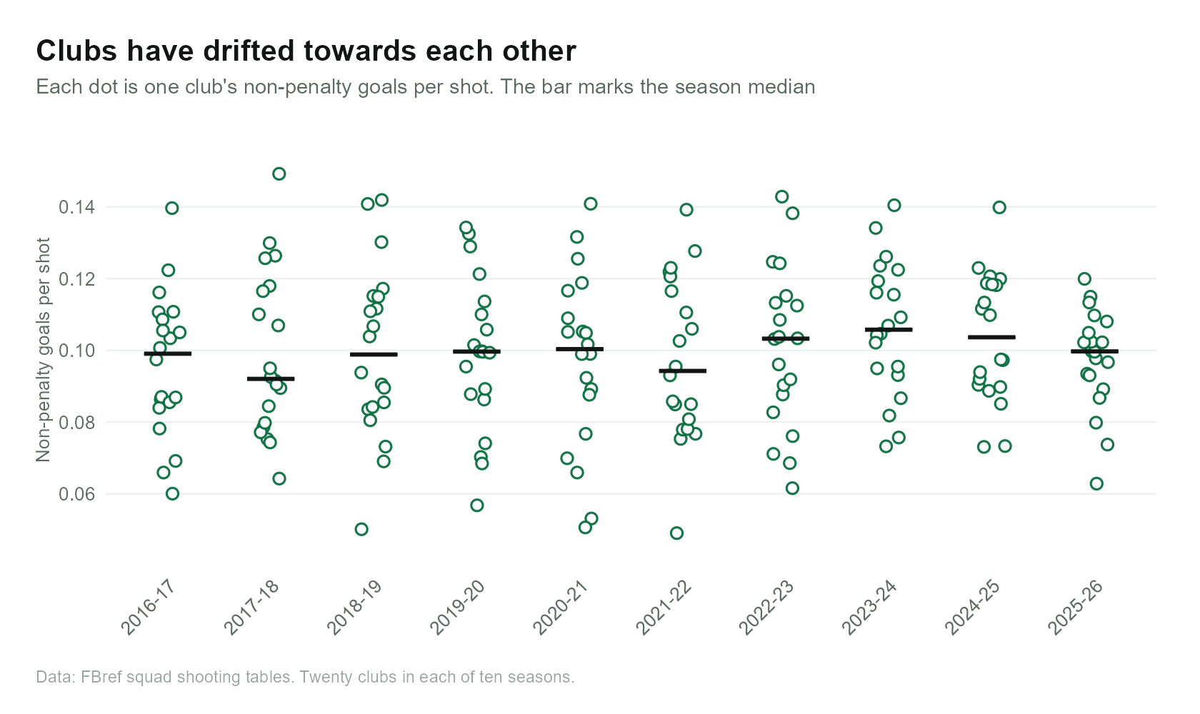
The first two pieces observed the league average and almost nothing moved. This article asks something different: not where the average was, but how the clubs were spread around the average.

What a club's own randomness looks like

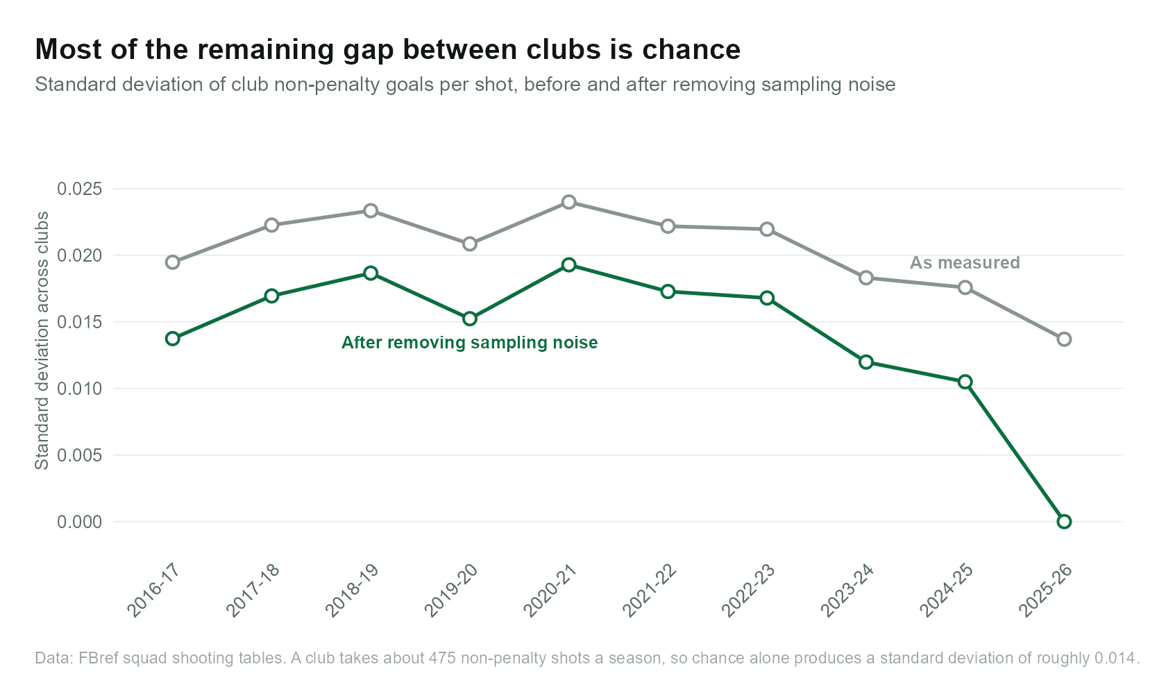
A club takes approximately 474 non-penalty shots in a season and scores about once in every ten attempts. Even if all twenty clubs were identical, that many attempts would produce different conversion rates by chance alone. That spread has a standard deviation of about 0.014.

That is, the measured differences between clubs mix real ability with chance, and the two cannot be told apart until the chance component is removed.

Club non-penalty goals per shot for each of ten seasons; the spread narrows in the last three. — **Fig 1** — The clubs got closer to each other. The spread was widest in 2020-21 and narrowest in the last season.

The spread has narrowed

Season	As measured	Chance alone	After correction
2016-17	0.0195	0.0138	0.0137
2017-18	0.0223	0.0144	0.0170
2018-19	0.0234	0.0140	0.0187
2019-20	0.0209	0.0142	0.0152
2020-21	0.0240	0.0143	0.0193
2021-22	0.0222	0.0139	0.0173
2022-23	0.0220	0.0142	0.0168
2023-24	0.0183	0.0138	0.0120
2024-25	0.0176	0.0141	0.0105
2025-26	0.0137	0.0139	0.0000

The slope before correction is −0.00066 per season (R² = 0.401), and the slope after correction is −0.00121 per season (R² = 0.415). The corrected spread peaked at 0.0193 in 2020-21, fell to 0.0105 by 2024-25, and in 2025-26 was indistinguishable from zero.

Standard deviation of club conversion rates by season, before and after removing sampling noise. — **Fig 2** — The distance between the two lines is the part chance produces. In 2025-26 it accounts for all of the measured spread.

Two ways of checking

The correction relies on an assumption that the variation by chance is p(1 − p) / n per club. So I checked twice instead of trusting the algebra.

Simulation. Twenty identical clubs each toss a coin as many times as that club's actual shot count, and the procedure is replicated 3,000 times. The standard deviation this produces matches the value the formula predicts to within 0.0005.

Chi-square test of homogeneity (df = 19; critical value at the 5% level = 30.1):

Season	X²	p
2018-19	56.7	0.0000
2022-23	51.1	0.0001
2023-24	35.2	0.0131
2024-25	30.3	0.0475
2025-26	18.8	0.4681

They are entirely different methods but state the same thing: only 2025-26 falls below the critical value.

How much of this rests on one season

I apply the standard I set in the first piece to my results.

Window	Slope after correction	R²
All ten seasons	−0.00121	0.415
Dropping 2025-26 (nine)	−0.00049	0.203
Dropping both end seasons (eight)	−0.00090	0.506

Excluding 2025-26, the trend weakens to less than half. It does not disappear, and remains even in the intermediate interval. But it relies heavily on the last season.

What this does not settle

This analysis does not settle four things:

I cannot say why the clubs converged. The data only shows that they did.
The result of 2025-26 is "indistinguishable in this sample", not "the teams are the same".
I only observed the conversion rate. The position and quality of the shots remain impossible to check.
It is a single league with ten seasons.

What's next

In the next article, I am going to analyze whether shot-on-target percentage predicts goals per shot, using a regression across 200 club-seasons.

Data and code. All ten CSV exports and the R script that produced these figures are in this site's repository.